
There *is* a smarter way to write Excel VLOOKUP formulas for financial analysis.
The title of this post really should have been “are you still using VLOOKUP?”, but I already know the answer to that question.
If you work in financial services, VLOOKUP is probably the most used function (yes, still), second only to IF. Yet I’ve seen some behemoth spreadsheets bogged down with many thousands of VLOOKUP formulas.
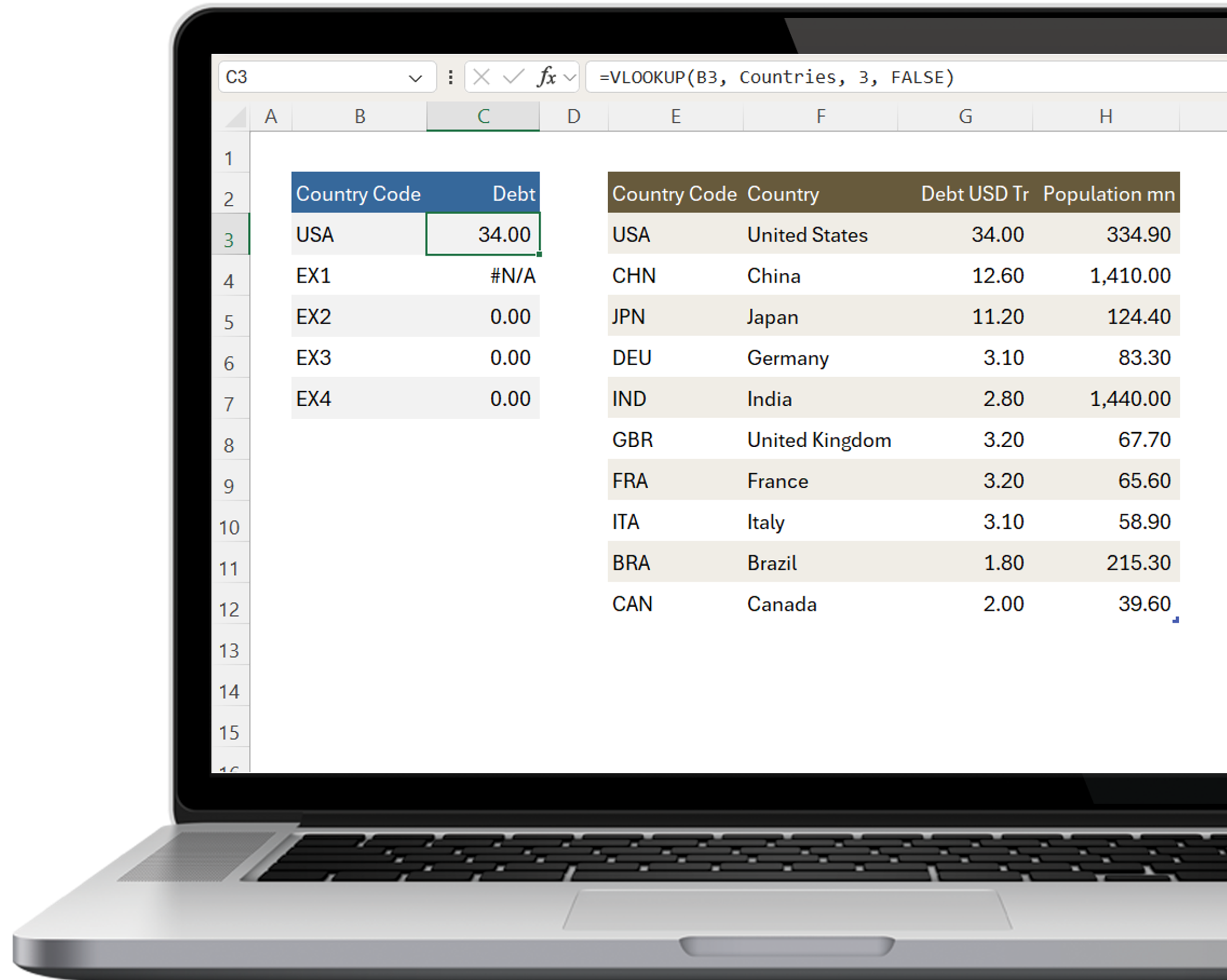
The Classic VLOOKUP
This is the classic VLOOKUP we’re so familiar with.
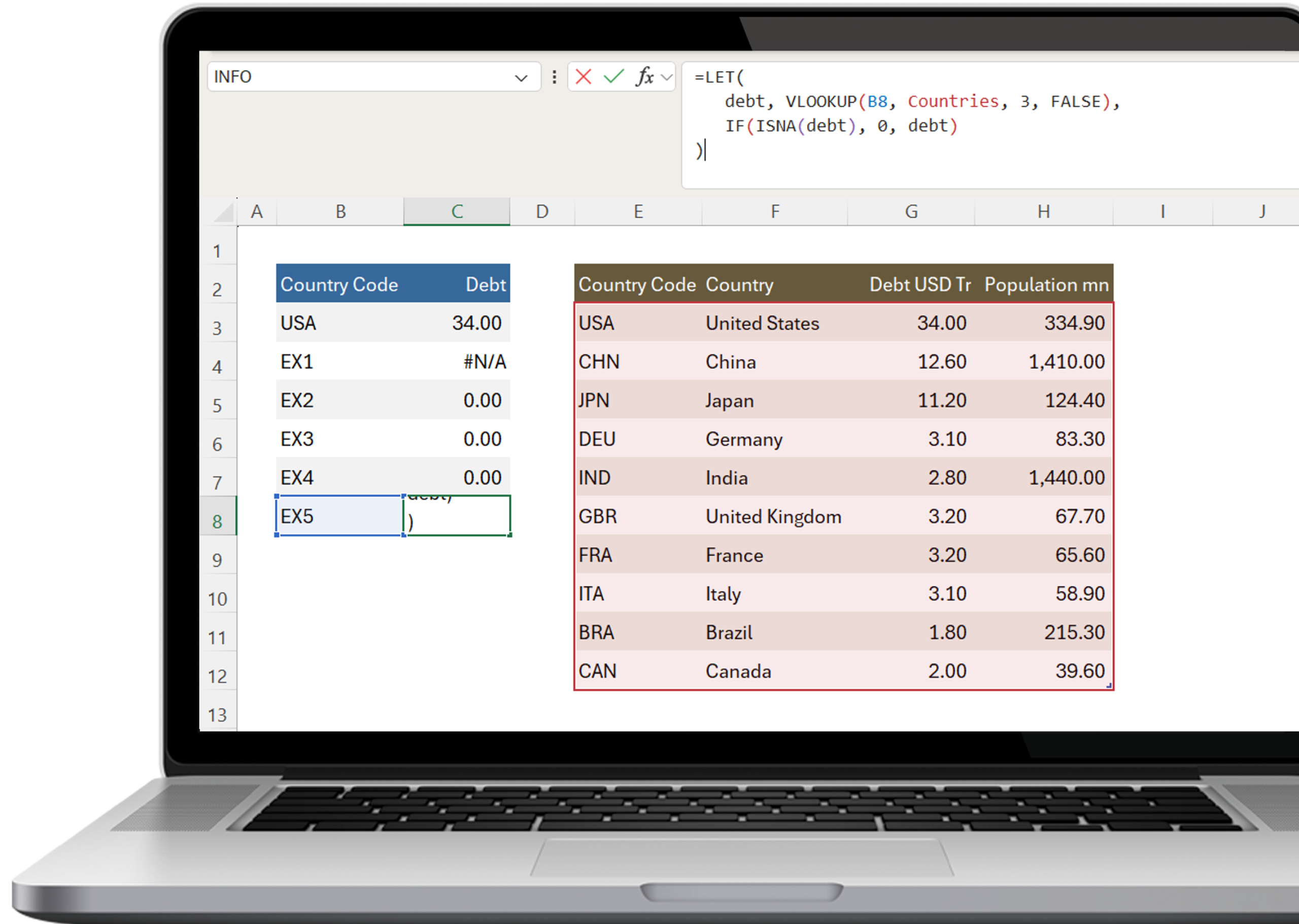
Look up the value in cell B3 in a table called Countries (you are using Excel Tables, aren’t you?) and return what’s in column 3.
Simples.
Works fine until the lookup value isn’t found. The you get the dreaded #N/A error.
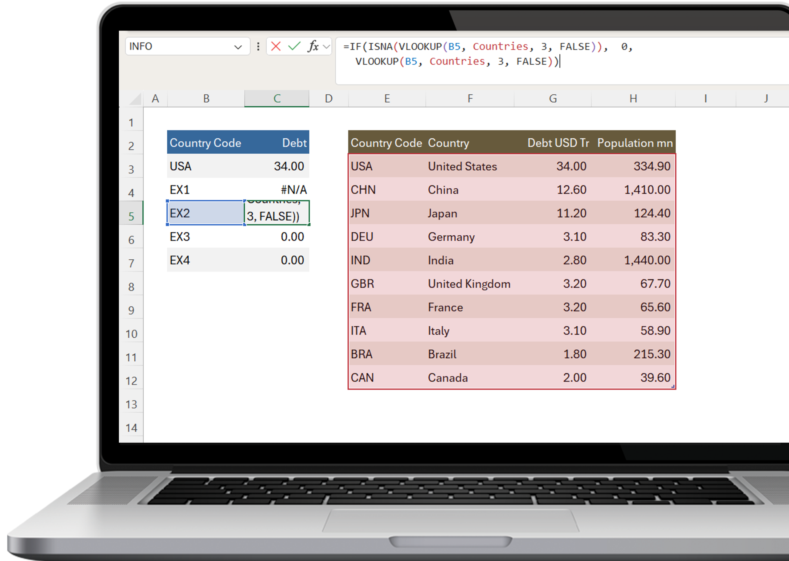
Double VLOOKUP
Unfortunately, a common way I’ve seen this resolved is by doubling down on VLOOKUP with an ISNA() function.
That is lookup up a value, if it doesn’t return #NA, look it up again.
Madness.
In small workbooks, this isn’t a big deal, but I’ve seen Excel workbooks grind to a halt with tens-of-thousands of doubled-up VLOOKUP formulas.
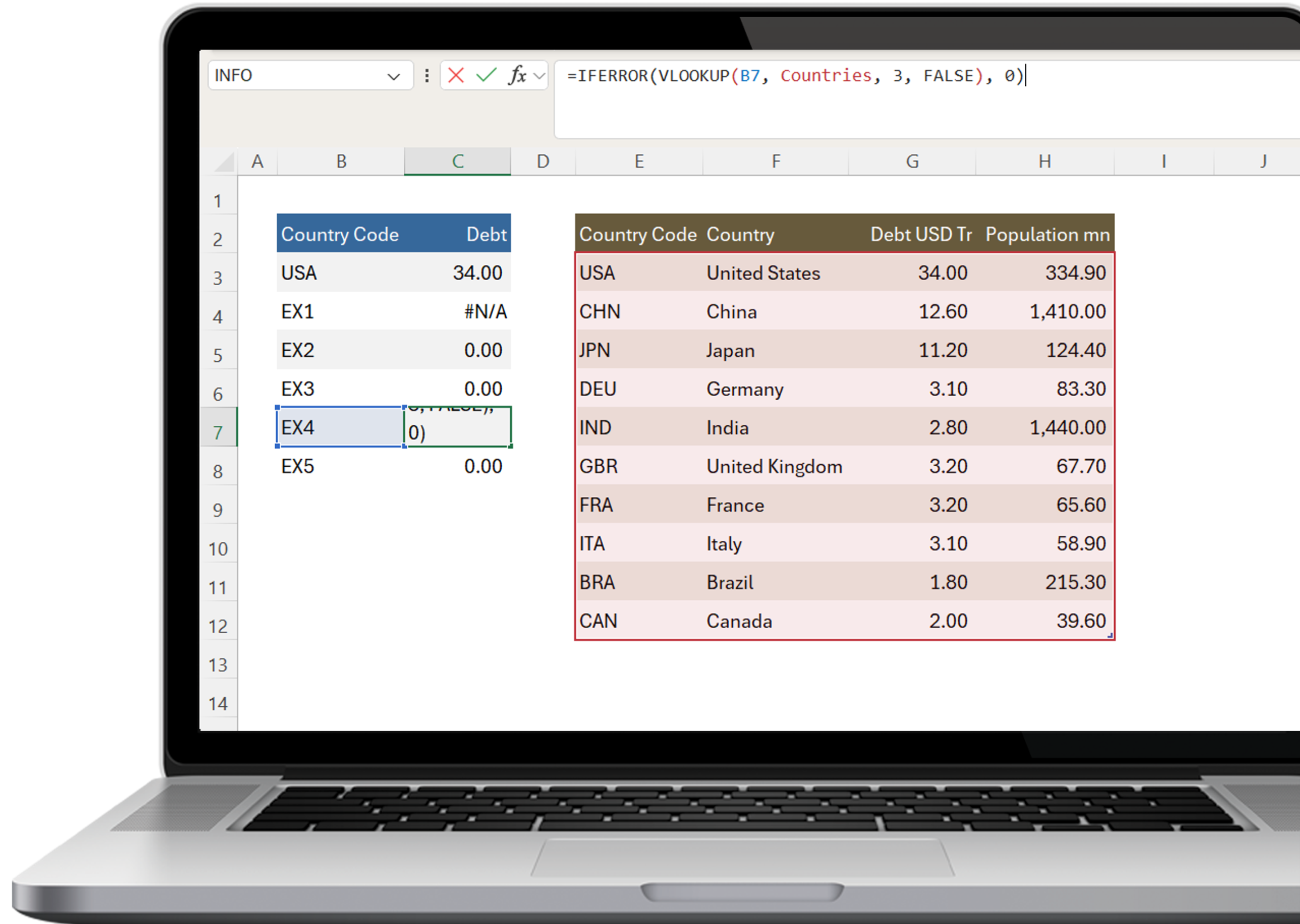
IFERROR is ‘better’
A more efficient fix is the IFERROR function.
IFERROR lookups up the value once and gives you the option of assigning an alternative value if an error occurs.
But . . .
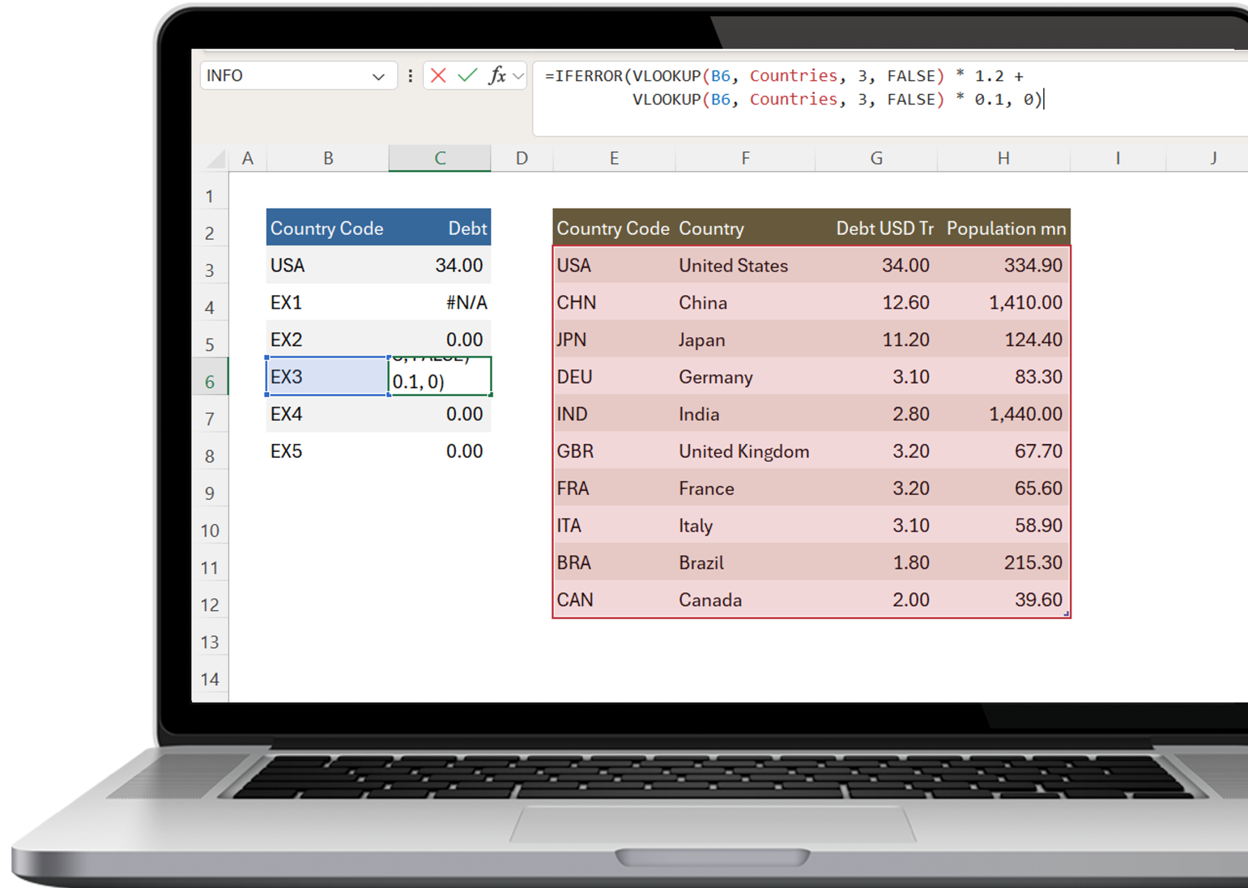
Multiple Lookups
IFERROR can still get messy and hide errors with multiple lookups to the same data.
This happens when:
LET to the Rescue
Try LET().
LET allows you to assign names to calculation results inside a formula.
This improves readability, performance and maintenance, especially if you use the same looked-up value multiple times.
Let has many benefits:
LET isn’t just for VLOOKUPS, it allows you to create simpler, yet more powerful formulas especially when they reference the same values multiple times.
Over to You
Over to you. Have you tried LET? How did it work out? Leave a comment below.
0 comments